Understanding Calibration Curves: A Comprehensive Guide for Beginners

Calibration curves are an important tool in analytical chemistry that allow scientists and technicians to determine the concentration of unknown samples. This is achieved by comparing the results from a known set of standards with the results from the unknown samples. In this article, we will discuss why we need calibration curves, how to build a calibration curve, and what materials are required for this process.

Why Do We Need Calibration Curves?

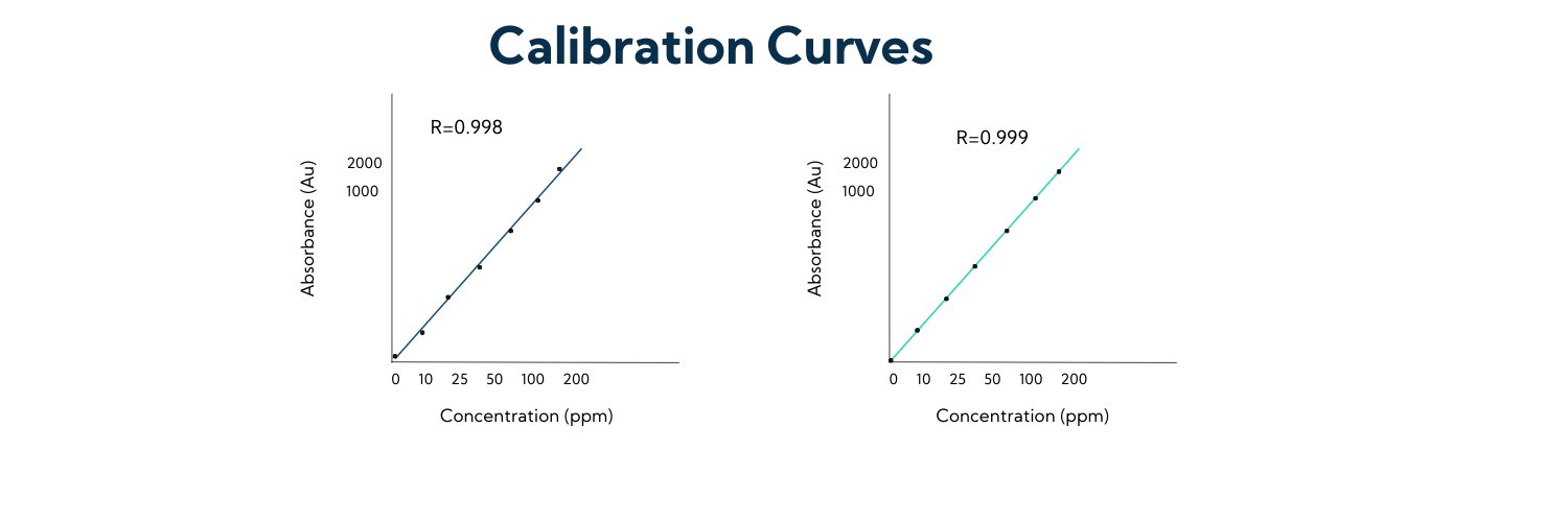
When a sample is injected into an analytical instrument such as an HPLC, the instrument generates an absorbance reading. However, this reading alone does not provide any information about the concentration of the sample. To determine the concentration, a calibration curve must be constructed. This is done by injecting a known set of standards into the instrument and using the results to compare against an unknown set of samples. The results from the known set of standards can then be used to extrapolate the values of the unknown samples.

For example, let’s say we have a 100 ppm standard and a 200 ppm standard, which generate roughly 1000 and 2000 absorbance units, respectively. If we have an unknown sample that generates 1500 absorbance units, we can be confident that it is approximately 150 ppm.

Building a Calibration Curve

To build a calibration curve, we need to start with a neat standard, which is a pure sample at a concentration of one million parts per million (ppm). We then create a stock solution, which is typically around 1000 ppm, from which we can dilute to our desired concentrations of 200 ppm, 100 ppm, etc.

The following materials are required to build a calibration curve:

Neat standard 

Metric flask for the stock solution

A set of 10 ml volumetric flasks for the individual calibration points

Transfer pipette

Spatula

Weigh boats

Balance

Pipette tips

To build a calibration curve, the following steps are taken:

Weigh out 200 mg of the neat standard and add it to a metric flask.

Top off the flask with water (or another solvent if necessary) to create a 2000 ppm stock solution.

Vortex the solution to mix it.

Transfer some of the stock solutions to a simulation vial for easy dilution.

Dilute the stock solution to your desired concentrations (200 ppm, 100 ppm, etc.) using temporal dilution.

Inject the standards into the HPLC and construct the calibration curve.

Note: In addition to the volumetric calibration curve, it is also possible to build a gravimetric calibration curve by weighing each step of the process.

Calibration curves are a critical tool in analytical chemistry that allows us to determine the concentration of unknown samples. Building a calibration curve requires a set of materials and a specific process, but the results can provide valuable information about the samples being analyzed.